Time normalization and GAM(M)s

Dec 6, 2022, LING 730

Wieling tutorial (tents/tenths)

Section 3:

Note that due to the fixed sampling rate (of 100 Hz) the number of sampling points per word is dependent on the word’s length. Our present dataset consists of 126,177 measurement points collected across 1618 trials (62 trials were missing due to sensor failure or synchronization issues). The average duration of each word (from the articulatory start to the articulatory end) is therefore about 0.78 seconds, yielding on average 78 measurement points per word production.

Section 4.1

The final two columns, Time and Pos, contain the normalized time point (between 0 and 1) and the associated (standardized) anterior position of the T1 sensor.

R Code, data set description:

Time - The normalized (between 0: beginning of the word, to 1: end of the word)

Soskuthy tutorial

Github repo

3.1 Analysing a simple simulated data set

The first data set contains simulated F2 trajectories, and is very similar to the example data set introduced in section 2.6.1. It contains 50 F2 trajectories, each of them represented by 11 measurements taken at equal intervals (at 0%, 10%, 20%, . . . , 100%). The observations in the data set are the individual measurements, which means that there are 550 data points altogether. The variable measurement.no codes the location of individual data points along the trajectory. Each of the trajectories has an ID (a number between 1–50), which is encoded in the column traj.

Note: tutorial also includes discussion of if AR(1) model can be used instead of random smooths by trajectory (or if you might need both!), see page 32:

it is important to look at residual autocorrelation plots and also to check how much variance is actually left in the residuals. There is, however, one practical consideration that makes the AR1 approach slightly more attractive. Adding an AR1 model to a GAMM is computationally inexpensive, while adding large numbers of random smooths can be very time- and memory-consuming. This may not be a problem for small data sets, but the computational cost of random smooths can be prohibitive for models with large numbers of trajectories. What if we still want to fit random smooths to a large data set? The function bam() has an optional argument discrete, which speeds up computation substantially when set to TRUE. Moreover, when discrete=TRUE, a GAMM can be fitted using multiple processor cores. The number of processor cores used in the computation is specified by the nthreads argument. Note that this technique only works with the fREML fitting method, so evaluating significance through model comparison may not be possible.

Section 4: Vowels over time data analysis

The data set consists of F3 trajectories measured at 11 evenly spaced points. The trajectories include both /r/ and the preceding vowel.

It seems that where "absolute time" comes in is via duration variable, see plots on pages 25 and 36

• Page 25: duration smooth as well as in interaction with measurment number

words.50.gam.dur <- bam(f2 ~ word.ord + s(measurement.no, bs="cr") + s(duration, bs="cr") + ti(measurement.no, duration) + s(measurement.no, by=word.ord, bs="cr"), data=words.50, method="ML")

• Page 36: duration smooth as well as in interaction with measurement number

gl.r.gamm.covs.2 <- bam(f3 ~ stress + s(measurement.no) + s(measurement.no, by=stress) + s(duration) + ti(measurement.no, duration) + s(decade, k=4) + ti(measurement.no, decade, k=c(10,4)) + s(measurement.no, speakerStress, bs="fs", m=1, k=4), dat=gl.r, method="ML")

EEG?

Referenced in autocorrelation paper by Baayen et al.

Nope: constant sampling rate, time-locked, same analysis window.

https://www.frontiersin.org/articles/10.3389/fpsyg.2015.00077/full#FA1

RT-MRI Labphon paper 2020

2.3. Normalization procedures

The current study uses GAMMs to observe how a variety of factors might condition changes in aperture throughout the vocal tract over the time course of the vowel. However, before submitting the data to the GAMMs, both of these dimensions (time and space, i.e., grid line location within the VT) were normalized. Time was normalized in a linear fashion for each token (scale: 0–1).

Tone data

Section 4

To capture the pitch contour of T1, the F0 values at ten equally-spaced time points of each target syllable were measured.

page 12-13

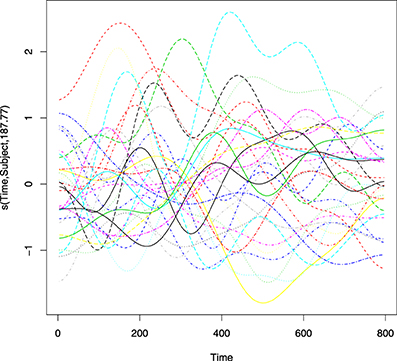
Before fitting models, we centered time. Time is a numeric variable ranging from one to ten in normalized time. Centering was implemented because the model intercept, the y-coordinate where the regression line hits the y-axis, is not interpretable, since pitch at time 0 does not make sense. We centered time so that the intercept now will represent the mean pitch in the middle of the arget syllables. We fitted our first model with sex, location, and context as fixed-effect factors, along with a smooth for the variable of scaled time (timeScaled). In addition, we also requested a by-subject factor smooth for timeScaled (i.e., a wiggly line for each subject) and random intercepts for word.

Paleoenvironmental data with irregularly spaced time series

R code

Section 4.1: Small Water

Now the i.i.d. assumption has been relaxed and a correlation matrix, Λ, has been introduced that is used to model autocorrelation in the residuals. The δ15N values are irregularly spaced in time and a correlation structure that can handle the uneven spacing is needed (Pinheiro and Bates, 2000). A continuous time first-order autoregressive process (CAR(1)) is a reasonable choice; it is the continuous-time equivalent of the first-order autoregressive process (AR(1)) and, simply stated, models the correlation between any two residuals as an exponentially decreasing function of h (ϕh), where h is the amount of separation in time between the residuals (Pinheiro and Bates, 2000). h may be a real valued number in the CAR(1), which is how it can accommodate the irregular separation of samples in time. ϕ controls how quickly the correlation between any two residuals declines as a function of their separation in time and is an additional parameter that will be estimated during model fitting.

Also see "adaptive smoothness" section. Section 4.7

While there is not much we can do within the GAM framework to model a series that contains both smooth trends and step-like responses, an adaptive smoother can help address problems where the time series consists of periods of rapid change in the mean combined with periods of complacency or relatively little change

Dealing with time series of varying lengths

• tslearn Methods for variable-length time series (Python)

  • "Finally, if you want to use a method that cannot run on variable-length time series, one option would be to first resample your data so that all your time series have the same length and then run your method on this resampled version of your dataset. Note however that resampling will introduce temporal distortions in your data. Use with great care!"

  • See other methods mentioned

  • Shapelets github discussion

    • Note two ways of getting equal length time series: would we ever want to pad?

      

• Clustering, see Table 4

• See gap filling section in tutorial from Rossiter (Cornell)

• Turn to frequency domain, e.g., do Fourier transform

• Other suggestions Quora

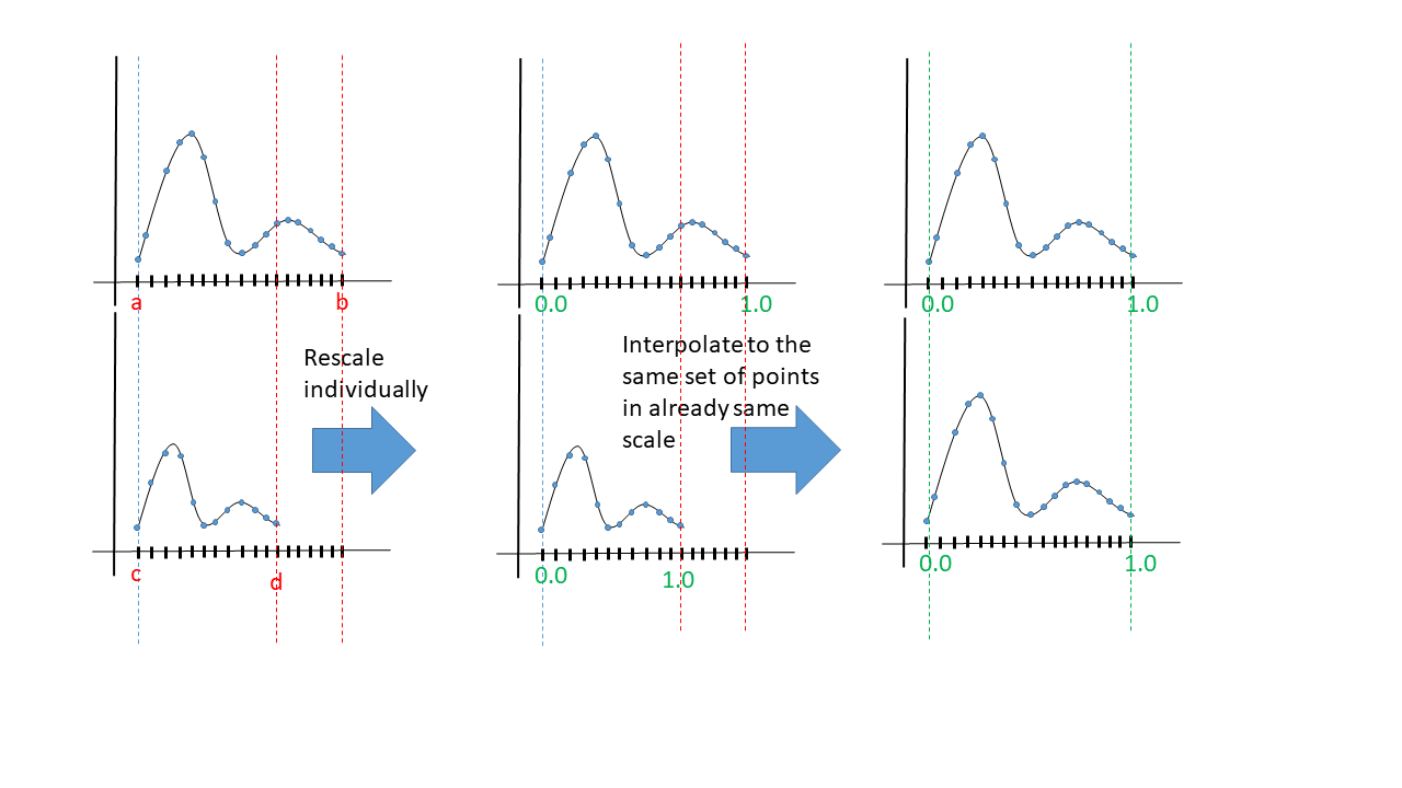
  • 1. Interpolation: Create a fixed length sample from each sample by using interpolation/curve fitting such as splines.
    2. Dynamic Time Warping or such. i.e. use length invariant models/classifiers.
    3. Create length independent features: use features that are length invariant, such as average, number of modes, features on the frequency domain etc.
    4. Use predefined time windows: Always look at fixed window sizes, and search for your patterns there. There are more advanced methods that look in parallel in windows of different lengths.

• Beyond Dynamic Time Warping? (for alignment of two time series)

  • Uniform Scaling and see helpful blog post, and slides, that explain upsampling via duplication of points

• Time series classification for varying length series (section 4)

  • Uniform scaling: "It rescales one series to the length of the other. It is more common to stretch the shorter series than to shrink the longer, because shrinking entails data loss"

  • "Low amplitude noise padding at the suffix of the time series": "This technique preserves the shape and does not change the information in the original series"

  • Low amplitude noise padding at the prefix and suffix of the time series

    • "This technique assumes that the longer time series has the complete pattern of an event that it is measuring and when the prefix and suffix of the shorter time series is padded with noise, the time series is “shifted” into the middle of the longer time series"

  • Single zero padding at the prefix and suffix of the time series

    • "However, unlike the previous techniques, it is important to be noted that this technique does not make the time series equal length. This is a new variant of prefix and suffix padding proposed in this work. It is inspired by the fact that it is common practice to z-normalize each time series to N (0, 1) before classification (Rakthanmanon et al., 2012; Ratanamahatana and Keogh, 2005). As the mean of the time series is zero, padding the prefix and suffix with a single zero allows DTW to align any number of leading and trailing points to this padded point with minimum expected cost. It also reduces unintuitive alignments between the two time series by relaxing the DTW constraint that the first and last point of the two time series must be aligned."

FPCA/GAMMs combos

Functional regression models (Puggaard-Rode 2022, JPhon)

Functional regression models are suitable when one or more variables are of a functional nature (Bauer et al., 2018). If an independent variable is functional and the response variable is constant over the functional domain, this can be modeled with scalar-on-function regression. This could e.g. be useful for researchers seeking to predict reaction times from pitch contours (e.g. Cutler, 1976); pitch contours consist of complex functional data, which will otherwise have to be either simplified or tightly controlled in the experimental set-up. If the response variable is functional and all independent variables are constant over the functional domain, this is suitably modeled with function-on-scalar regression. This, in contrast, could be useful for researchers seeking to predict the shape of pitch contours from a range of predictor variables, such as pragmatic context or duration. It is likewise useful for modeling how the spectrum of a speech sound is affected by e.g. contextual variables, as I will show below

In a model of spectral variance formalized in mgcv, the response variable would have to be an amplitude measure, whereas in a model formalized in refund, the response variable can be the spectral shape, which is conceptually more satisfactory.

What happened to landmark registration??

https://arxiv.org/abs/2203.14810

Elastic FPCA (updated packages) https://cran.r-project.org/web/packages/fdasrvf/fdasrvf.pdf